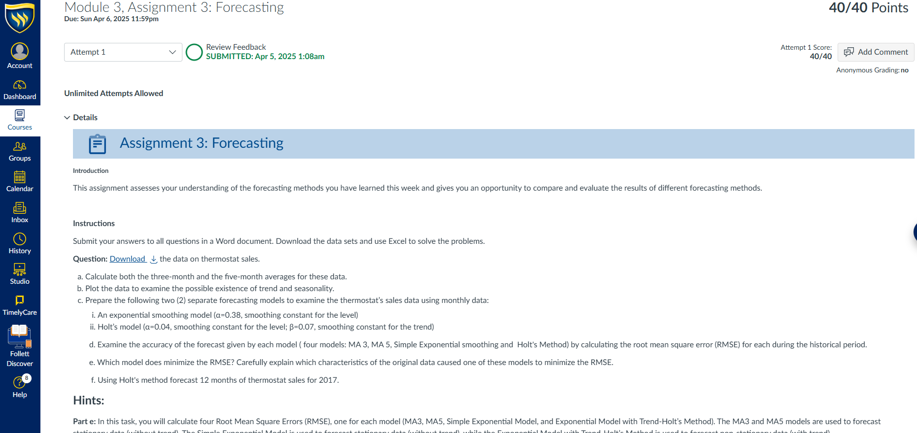
Need Help ?

Our Previous Samples

ECO 6214 : Module 5, Assignment 5: Forecasting | Due: Sun Apr 20, 2025 11:59pm ...

ECO 6214 : Module 5, Assignment 5: Forecasting

Introduction

This assignment assesses your understanding of and ability to apply multiple regression models to a series of business data using the Excel Analysis ToolPak.

Instructions

Submit your answers to all of the questions in a Word document. Download the data sets and use Excel to solve the problems.

Question 1. Download the data and develop a multiple-regression model for auto sales as a function of population and household income for 10 metropolitan areas.

  1. Estimate values for b0, b1, and b2 for this model:
    AS = b0 + b1 (INC) + b2 (POP)
  2. Are the signs you find for the coefficients consistent with your expectations? Explain.
  3. What percentage of variation in AS is explained by this model?
  4. What point estimate of AS would you make for a city where INC=23,175 and POP=128.7?

Question 2. The quarterly sales of the TRK-50 mountain bike for the previous four years by a bicycle shop in Switzerland are presented in the table:

Year Quarter Q = Sales
2010 1 10
  2 31
  3 43
  4 16
2011 1 11
  2 33
  3 45
  4 17
2012 1 13
  2 34
  3 48
  4 19
2013 1 15
  2 37
  3 51
  4 21


  1. Plot the sales against time.
  2. Use the data to estimate the monthly trend in sales using a linear trend model of the form:
    Qt = a + bt. Does your statistical analysis indicate a trend? If so, is it an upward or downward trend and how great is it? Is it a statistically significant trend at 5 percent level of significance?
  3. Now adjust your statistical model to account for seasonal variation in sales. Estimate this model of sales:
    Qt = a + bt + cD2 + dD3 + eD4
    where D2, D3, D4 are the appropriately defined dummy variables for quarters 2, 3, and 4.
    Do the data indicate a statistically signifi¬cant seasonal pattern at 5 percent level of significance? If so, what is the seasonal pattern of sales?
  4. Comparing your estimates of the trend in sales in parts b and c, which estimate is likely to be more accurate? Why?
  5. Using the estimated forecast equation from part c, forecast sales for Quarters 1 and 4 of 2014 and Quarters 2 and 3 of 2015.

Submission

  • Submit your answers in a Word document.
  • Submit the Excel files to show your calculations.
  • Include the relevant graphs of actual and forecast values of the series. Please do not forget to title your graph.

Submit your calculations and answers in a 1–3-page document and spreadsheet to the Dropbox by Day 7 of the week.


READ MORE >>

ECO 6214 : Module 5, Discussion: Dummy Variables ...

ECO 6214 : Module 5, Discussion: Dummy Variables

Introduction

This discussion provides you with an opportunity to discuss the use of dummy variables for capturing seasonality in the data.

Instructions

Respond to these questions:

  • Explain what dummy variables are and how they can be used to account for seasonality.
  • Please cite at least one academic article (APA or MLA format). 
  • Select a product or service of your choice and explain how you would use dummy variables to measure seasonality in the sales of that product or service.
  • Explain the expected sign of each dummy variable.

Directions

  • Make your initial post by Day 4 of this week and comment on at least two of your classmates’ posts by Day 7.
  • Post your response to the discussion and then read your classmates’ posts. Post TWO responses to at least TWO of your classmates' posts. Initial post should be no less than 150 words and no more than 450 words.
  • Discussions need to be professional. Please make proper use of capitalization and punctuation and make sure that there are no misspellings, incomplete sentences, or other grammatical errors.
  • The basic criterion for a discussion post to be considered effective is that your message is original and intelligible. You must communicate concisely and clearly.


READ MORE >>

ECO 6214 : Module 4, Assignment 4: Forecasting | Due: Sun Apr 13, 2025 11:59pm ...

ECO 6214 : Module 4, Assignment 4: Forecasting

Introduction

This assignment assesses your understanding of the simple linear regression model and provides you with an opportunity to apply this method to forecast data.

Instructions

Submit your answers to all questions in a Word document. Download the data sets and use Excel to solve the problems.

Question 1. Carolina Wood Products, Inc., a major manufacturer of household furniture, is interested in predicting expenditures on furniture (FURN) for the entire United States. You are going to help the company with this prediction. Download the data by quarter for 2007 through 2016.

  1. Estimate the bivariate linear trend model for the data where TIME=1 for 2007, Q1 through TIME=40 for 2016, Q4.

    FURN = a + b(TIME)

  2. Evaluate this model in one paragraph, with particular emphasis on its usefulness in forecasting.
  3. Prepare a time-trend forecast of furniture and household equipment expenditures for 2017 based on the model in (b).
    Period Time Trend Forecast
    2017 Q1 41
    2017 Q2 42
    2017 Q3 43
    2017 Q4 44


Question 2. Alexander Enterprises manufactures plastic parts for the automotive industry. Download data on its sales (in thousands of dollars) for 2012, Q1 through 2016, Q4. You are to forecast sales for 2017, Q1 through 2017, Q4.

  1. Begin by preparing a time series plot of the data set. Does it appear from this plot that a linear trend model will be appropriate? Explain. (Attach your graph to your answer.)
  2. Use a bivariate linear regression trend model to estimate this trend equation:
    SALES = a + b(TIME)
    Is the sign of b what you would expect? Is b significantly different from zero? What is the coefficient of determination for this model? Explain your answers.
  3. Based on this model, make a trend forecast of sales (SALESFT) for the four quarters of 2017.
  4. The actual sales (SALESA) for the four quarters are provided in the table.
    2017, Q1 4447.1
    2017, Q2 4501.6
    2017, Q3 4543.2
    2017, Q4 4603.1


Calculate RMSE for this forecast model in the historical period (2012, Q1–2016, Q4) as well as for the forecast horizon (2017, Q1–2017, Q4). Which of these measures accuracy and which measures fit?

Submission

  • Submit your answers in a Word document.
  • Submit the Excel files to show your calculations.
  • Include the relevant graphs of actual and forecast values of the series. Please do not forget to title your graph.

Submit your calculations and answers in a 1–3-page document and spreadsheet to the Dropbox by Day 7 of this week.


READ MORE >>

ECO 6214 : Module 4, Discussion: House Sales Forecast with Bivariate Regression ...

Introduction

This discussion allows you to discuss and apply the linear trend model for forecasting total house sales in the United States.


Instructions

Download the data on annual historical total houses sold (THS) in the U.S. and its regions. Select a region you are interested in and get the last 20 years of data.

To prepare for the discussion, undertake the analysis on the given points:

  • By using a bivariate regression trend line model, forecast total houses sold for the next five years.
  • Prepare a time series plot of these data (years are on the x axis, THS is on the y axis) that shows both actual and forecast THS for the next five years.

Post the results of your statistical analysis and the graph with your response to the following:

  • Do you think the model looks as though it will provide reasonably accurate forecasts for a five-year horizon? Explain your answer.

HINTS:

  • The data set in the discussion includes multiple spreadsheets. You will need to use the data on the first spreadsheet (Sol Ann). Choose a region from this spreadsheet and extract 20 years of house sales data (1996-2016). Next, use a linear trend model to forecast the next five years.
  • I have also created a video demonstrating the use of a linear trend model with Texas population data. Please watch the video, and if you have any questions, please let me know.

Linear Trend Model with Texas Population Data.


  • Refer to the given video if you do not know how to estimate data with a trend line in Excel.

Corman, L. (2010, September 28). Trend lines and regression analysis in excel. [Video file] [14 min 43 sec]. Retrieved from https://www.youtube.com/watch?v=6rOlGbLeQxI

Directions

  • Make your initial post by Day 4 of this week and comment on at least two of your classmates' posts by Day 7.
  • Post your response to the discussion and then read your classmates’ posts. Post TWO responses to at least TWO of your classmates' posts. Initial post should be no less than 150 words and no more than 450 words.
  • Discussions need to be professional. Please make proper use of capitalization and punctuation and make sure that there are no misspellings, incomplete sentences, or other grammatical errors.
  • The basic criterion for a discussion post to be considered effective is that your message is original and intelligible. You must communicate concisely and clearly.


Expert Answer


READ MORE >>

ECO 6214 : Module 3, Assignment 3: Forecasting ...

ECO 6214 : Module 3, Assignment 3: Forecasting

Introduction

This assignment assesses your understanding of the forecasting methods you have learned this week and gives you an opportunity to compare and evaluate the results of different forecasting methods.


Instructions

Submit your answers to all questions in a Word document. Download the data sets and use Excel to solve the problems.

Question: Download the data on thermostat sales.

  • Calculate both the three-month and the five-month averages for these data.
  • Plot the data to examine the possible existence of trend and seasonality.
  • Prepare the following two (2) separate forecasting models to examine the thermostat’s sales data using monthly data:
    • An exponential smoothing model (α=0.38, smoothing constant for the level)
    • Holt’s model (α=0.04, smoothing constant for the level; β=0.07, smoothing constant for the trend)

        d. Examine the accuracy of the forecast given by each model ( four models: MA 3, MA 5, Simple Exponential smoothing and  Holt's Method) by calculating the root mean square error (RMSE) for each during the historical period.

        e. Which model does minimize the RMSE? Carefully explain which characteristics of the original data caused one of these models to minimize the RMSE.

         f. Using Holt's method forecast 12 months of thermostat sales for 2017.

Hints:

Part e: In this task, you will calculate four Root Mean Square Errors (RMSE), one for each model (MA3, MA5, Simple Exponential Model, and Exponential Model with Trend-Holt’s Method). The MA3 and MA5 models are used to forecast stationary data (without trend). The Simple Exponential Model is used to forecast stationary data (without trend), while the Exponential Model with Trend-Holt’s Method is used to forecast non-stationary data (with trend).

Visualizing the data will help you detect any data patterns such as trend, seasonality, or stationary data with random errors. This will assist you in answering part e of the task.

Part f: In the lecture notes, the embedded video on Holt's Method did not explain how to forecast future data using Holt's Method. To forecast with Holt's Method, use the following algebraic form:

Ht+m = Ft+m * Tt

Here, Ht+m represents Holt’s forecast value for period t+m. Please watch virtual lab 3 recordings to learn how to complete this part.

Virtual Lab 3.

Assignment 3's dataset is larger than the previous assignments, and thus, you can limit the amount of data that you report in the Word document by following the instructions below:

Part A: Report a table that includes the last five periods of forecast (MA3 and MA5), including January 2017. Alternatively, you can include a plot of actual and forecast data.

Part B: Include a plot of actual data along with an explanation.

Part C: Report a table that includes the last five periods of forecast (Simple Exponential Smoothing and Holt's), including January 2017. Alternatively, you can include a plot of actual and forecast data. Please refer to the videos I posted to make a forecast with Simple Exponential Smoothing and Holt's.

Part D: Report the RMSE's of all four models.

Part E: Provide an explanation.

Part F: Include a table that shows a 12-month forecast with Holt's Method.


Submission

  • Submit your answers in a Word document.
  • Submit the Excel files to show your calculations.
  • Include the relevant graphs of actual and forecast values of the series. Please do not forget to title your graph.

Submit your calculations and answers in a 1–3-page document and spreadsheet to the Dropbox by Day 7 of this week.


READ MORE >>

ECO 6214 : Module 3, Midterm Exam ...

Module 3, Midterm Exam

Attempt 1   Score for this quiz: 90 out of 120
Submitted Apr 6 at 7:16pm
This attempt took 32 minutes.


Question 1                                     10 / 10 pts
Under what circumstances may it make sense NOT to prepare a business forecast?
  

  • No data is readily available.  
  • There is no consensus among informed individuals.  
  • The industry to forecast is undergoing dramatic change.  
  • The future will be no different from the past.  
  • The forecast horizon is 40 years.

 
Question 2                        5 / 5 pts
Which subjective forecasting method depends upon the anonymous opinion of a panel of individuals to generate sales forecasts?  

  • None of the above.
  • Sales Force Composites.
  • Jury of Executive Opinion.
  • Customer Surveys.
  • Delphi Method.

 
Question 3                              5 / 5 pts
Which of the following is NOT considered a subjective forecasting method?

  •   Consumer surveys.
  •   Juries of executive opinion.
  •   Sales force composites.
  •   Naive methods.
  •   Delphi methods.

 
Question 4             5 / 5 pts
Suppose you are attempting to forecast a variable that is independent over time such as stock rates of return. A potential candidate-forecasting model is
  

  • The Delphi Method.  
  • None of the above.  
  • The Jury of Executive Opinion.  
  • Last period’s actual rate of return.  
  • Last period’s actual rate of return plus some proportion of the most recently observed rate of change in the series.

 
Question 5                               5 / 5 pts
Of the following model selection criteria, which is often the MOST important in determining the appropriate forecast method?

  •  Technical background of the forecast user.
  •  When is the forecast needed?
  •  What is the forecast horizon?
  •  Patterns the data have exhibited in the past.
  •  How much money is in the forecast budget?

 
Question 6                 5 / 5 pts
Which time-series component is said to fluctuate around the long-term trend and is fairly irregular in appearance?

  •   Cyclical.
  •   Irregular.
  •   None of the above.
  •   Seasonal.
  •   Trend.

 
Question 7                                      10 / 10 pts
For which data frequency is seasonality not a problem?

  •   Annual.
  •   Daily.
  •   Monthly.
  •   Weekly.
  •   Quarterly.

 
Question 8                                            5 / 5 pts
When a time series contains no trend, it is said to be

  •   nonseasonal.
  •   seasonal.
  •   nonstationary.
  •   stationary.
  •   filtered.

 
Question 9             10 / 10 pts
A large sample of X-Y data values are analyzed and reveal a correlation coefficient of-.88. Which statement is correct?

  •   The correlation is weak because r is less than -1.
  •   There is no relation. 
  •   A weak negative relationship exists.
  •   A fairly strong negative linear relationship exists. *
  •    If r had been +.88, the correlation would have been much stronger.

 
Question 10                      10 / 10 pts
Which method uses an arithmetic mean to forecast the next period?

  •   Exponential smoothing.
  •   Adaptive filtering.
  •   Moving averages.
  •   None of the above
  •   Naive.

 
Question 11                            10 / 10 pts

Time Period

Actual Series

Forecast Series

Forecast Error

1

100

100

0

2

110

--

--

3

115

--

--


If a three-month moving-average model is used, what is the forecast for period 4?

  •   107.1.
  •   108.3.
  •   110.2.
  •    106.6.
  •   104.4.

 
Question 12                      10 / 10 pts

Time Period

Actual Series

Forecast Series

Forecast Error

1

100

100

0

2

110

--

--

3

115

--

--

If a smoothing constant of .3 is used, what is the exponentially smoothed forecast for period 3?

  •   103.0.
  •   106.6.
  •   115.0.
  •   104.4.
  •   112.6.

 
Question 13                                     10 / 10 pts

The ACF for The Gap sales is shown above. There is clear evidence in the ACF that

  •   Gap sales have fallen in the last 12 periods.
  •   there is a strong trend in the data.
  •   the data is too strongly correlated to identify trend.
  •   the data is stationary.
  •   there is no seasonality in the data.

 
Question 14                        10 / 10 pts
If the correlation between body weight and annual income were high and positive, we could conclude that

  •   high incomes cause people to gain weight.
  •   high income people tend to be heavier than low income people, on average.
  •   low incomes cause people to eat less food.
  •   high incomes cause people to eat more food.
  •   high income people tend to spend a greater proportion of their income on food than low income people, on average.

 
Question 15                                  10 / 10 pts
In the Holt's two-parameter smoothing model, the trend smoothing parameter Gamma

  •   should be close to one when α is one.
  •   should be close to one when the data has a relatively smooth trend.
  •   should be close to one when α is close to one.
  •   should be close to zero when the data has a relatively smooth trend.

READ MORE >>

ECO 6214 : Module 2, Assignment 2: Forecasting ...

ECO 6214 : Module 2, Assignment 2: Forecasting

Introduction

This assignment will test your knowledge of basic statistical concepts, the components of time series data, and using a correlogram for model selection.


Instructions

Submit your answers to all questions in a Word document. Download the data sets and use Excel to solve the problems.

Question 1. Thirty graduate students were asked how many credit hours they were taking in the current quarter. Download the available dataDownload Download the available data

  1. Calculate the mean, median, standard deviation, variance, and range for this sample using Excel. Write a sentence explaining what each measure means.
  2. What is the standard error of the mean based on the data?
  3. What would be the best point estimate for the population credit hours? (“Population” refers to all graduate students’ credit hours in the universe.)
  4. What is the 95% confidence interval for the means of credit hours? What is the 90% confidence interval?

Question 2. An investment manager has been working on a report for forecasting Apple stock price. Your job is to help him to determine whether there is a trend and/or seasonality in Apple stock prices. Download the dataDownload Download the data

  1. Prepare a time series plot of these data.
  2. Include a trend line using the Excel Analysis ToolPak. On the basis of your analysis, do you think there is a significant trend in Apple stock prices? Explain.

Watch the following video to learn how to add a trendline:

Watch the video: How to Add a TrendlineLinks to an external site. 

  1. Is there seasonality? Explain.
  2. What forecasting method might be appropriate for Apple stock prices according to the guidelines provided in your Table 2.1 (Chapter 2, page 58) of your textbook?

Question 3. The given figure is the correlogram for the total number of houses in the U.S. (quarterly data).

correlogram for the total number of houses in the U.S

On the basis of the correlogram, do you think there is a significant trend? Explain.

Submission

  • Submit your answers in a Word document.
  • Submit the Excel files to show your calculations.
  • Include the relevant graphs of actual and forecast values of the series. Please do not forget to title your graph.

Submit your calculations and answers in a 1–3-page document and spreadsheet to the Dropbox by Day 7 of this week.


READ MORE >>

ECO 6214 : Module 2: Discussion: Trend and Seasonal Data Patterns ...

ECO 6214 : Module 2: Discussion: Trend and Seasonal Data Patterns

Introduction

This discussion will assess your ability to apply what you have learned this week using the sales data of a real company. You will also test your opinions and ideas against the ideas and opinions of your classmates.


Instructions

Select a corporation you are interested in and find that corporation’s annual reports for five consecutive years. Study these five annual reports and find the corporation’s total revenue (sales in dollar units) for each of those five years.

How to get sales data using Mergent online.

Perform the given tasks to prepare for the discussion:

  • Prepare a time series plot of these data (years on the x axis, sales on the y axis).
  • Use the first naive model you learned about in Week 1 to forecast data for year 6.
  • Plot the actual data along with your forecast data.

Post your graph with your answer to the given question:

  • Based on your graph of the actual data, do you think there is a trend in the data? Is there any seasonal variation? Please explain your reasoning.

Data sources and help with graphs

  • You can access the Mergent Online database using your Texas Wesleyan login information. Mergent Online contains annual reports of many public corporations.
  • The Yahoo! Finance Company and Fund Index offers company profiles, financial information, and links to a range of resources. Write the company name in the search bar and select the financials tab on the screen.
  • Watch the given video if you do not know how to plot data in Excel:

Directions

  • Make your initial post by Day 4 of this week and comment on at least two of your classmates’ posts by Day 7.
  • Post your response to the discussion and then read your classmates’ posts. Post TWO responses to at least TWO of your classmates' posts. Initial post should be no less than 150 words and no more than 450 words.
  • Discussions need to be professional. Please make proper use of capitalization and punctuation and make sure that there are no misspellings, incomplete sentences, or other grammatical errors.
  • The basic criterion for a discussion post to be considered effective is that your message is original and intelligible. You must communicate concisely and clearly.


Expert Answer

ANSWER TO : Module 2: Discussion: Trend and Seasonal Data Patterns


READ MORE >>

ECO 6214 : Assignment 1: Forecasting ...


ECO 6214 : Assignment 1: Forecasting 1

ECO 6214 : Assignment 1: Forecasting 2

Assignment 1: Forecasting

Introduction

This assignment will assess your knowledge of the concepts and techniques you have learned this week. Please answer the questions and submit your answers in a Word document.

Instructions

Submit your answers to both questions in a Word document. Download the data sets and use Excel to solve the problems.

Question 1. CoastCo Insurance is interested in developing a forecast of larceny thefts in the United States. Download the spreadsheet  for the available data.

  1. Plot this series in a time series plot and make a naive forecast for years 2 through 19. 
  2. Plot actual and forecast values of the series for the years 1 through 19. (You will not have an actual value for year 19 or a forecast value for year 1.)
  3. Calculate the RMSE  for years 2 through 18. On the basis of these measures and what you see in the plot, what do you think of your forecast? Explain. 

Watch the given video if you do not know how to plot data in Excel:

Igines. (2012, December 9). How to make a line graph in excel (scientific data). [Video file] [6 min 41 sec]. Retrieved from https://www.youtube.com/watch?v=Xn7Sd5Uu42A&t=1s


Question 2. As the world’s economies become increasingly interdependent, various exchange rates between currencies have become important in making business decisions. For many U.S. businesses, the European Union exchange rate (in euro per U.S. dollar) is an important decision variable. Download the spreadsheetwith the data on this exchange rate (EXEUR) by month for a two-year period.

  1. Prepare a time series plot of this data series.
  2. Use the naive forecasting model to forecast EXEUR for each month from year 1 M2 through year 3 M1.
  3. Plot actual and forecast values of the series for the year 1 M1 through year 3 M1. (You will not have an actual value for year 3 M1 or a forecast value for year 1 M1)
  4. Calculate RMSE for the period from year 1 M2 through year 2 M12. 

Other helpful Videos:

Plotting a series in a time series plot: A time series plot is a graph where time is the unit on the x-axis. The x-axis is labeled as the time-axis, and the y-axis represents the variable being measured. The x-values correspond to the time period, which can range from year 1 to year 18 for the first question and from year 2016 M1 to 2017 M12 for question 2. The y-values represent Larceny Theft for question 1 and EXEUR for question 2.

Plotting data in a time series plot. (1:36)

Plot actual and forecast values: In this plot, you are asked to graph two series together: the actual data and the forecast that you calculated. You can find an example of how to plot two series in a time series plot. The x-axis represents time, and the y-axis represents both actual and forecasted values. Here is a short video on how to plot actual and forecasted values in a time series plot:

Plot Multiple Lines in Exce. (1:56)

Submission

  • Submit your answers in a Word document.
  • Submit the Excel files to show your calculations.
  • Include the relevant graphs of actual and forecast values of the series. Please do not forget to title your graph.

Submit your calculations and answers in a 1–2-page document and spreadsheet to the Dropbox by Day 7 of this week.


READ MORE >>

ECO 6214 : Module 1, Discussion: Qualitative and Quantitative Forecasting Method ...

ECO 6214 : Module 1, Discussion: Qualitative and Quantitative Forecasting Methods

ECO 6214 : Module 1, Discussion: Qualitative and Quantitative Forecasting Methods


Introduction

You have now been introduced to qualitative and quantitative forecasting methods. Consider the advantages and disadvantages of these methods in this discussion activity.

Instructions

Respond to the given questions:

  • Compare what you think are the advantages and the disadvantages of subjective forecasting methods.
  • How do you think the use of quantitative methods relates to these advantages and disadvantages?
  • Please cite at least two academic articles (APA or MLA format).

Directions

  • Make your initial post by Day 4 of this week and comment on at least two of your classmates’ posts by Day 7.
  • Post your response to the discussion and then read your classmates’ posts. Post TWO responses to at least TWO of your classmates' posts. Initial post should be no less than 150 words and no more than 300 words.
  • Discussions need to be professional. Please make proper use of capitalization and punctuation and make sure that there are no misspellings, incomplete sentences, or other grammatical errors.
  • The basic criterion for a discussion post to be considered effective is that your message is original and intelligible. You must communicate concisely and clearly.


Expert Answer

Subjective forecasting methods can be valuable, especially when there is insufficient data to rely on. One of the most significant benefits is their flexibility—experts can adjust their forecasts based on new information or sudden changes, something quantitative methods can struggle with if there is no historical data to work from. These methods also bring in the insight of people with deep knowledge of the subject, which can be critical in situations where things are uncertain or complex to predict.
That said, subjective forecasting is not without its flaws. It is highly vulnerable to biases, like overconfidence or personal experience, which can skew predictions (Sharma, 2024). Unlike quantitative methods, measuring how accurate a subjective forecast is is complex, making it hard to trust in high-stakes scenarios.
Quantitative methods, on the other hand, are more reliable when there is solid data to work with. They are objective and consistent, which makes them great for stable situations (Verhoef & Casebeer, 1997). However, they can miss the bigger picture, especially in unpredictable environments or when qualitative factors matter. Ultimately, combining both approaches can often be the best way to go. Quantitative methods provide a data-backed starting point, while subjective insights can help fill in the gaps and adjust for the unknowns that data cannot always predict.

References:

1.  Sharma, G. (2024, March 19). Optimizing demand forecasting: Challenges and best practices. Institute for Supply Management. https://www.ismworld.org/supply-management-news-and-reports/news-publications/inside-supply-management-magazine/blog/2024/2024-03/optimizing-demand-forecasting-challenges-and-best-practices/Links to an external site.

2. Verhoef, M. J., & Casebeer, A. L. (1997, March). Broadening horizons: Integrating quantitative and Qualitative Research. The Canadian journal of infectious diseases = Journal canadien des maladies infectieuses. https://pmc.ncbi.nlm.nih.gov/articles/PMC3327344/Links to an external site.

3. Wilson, J. H., & Keating, B. (2018). Forecasting & predictive analytics: With ForecastX. McGraw-Hill/Irwin.


READ MORE >>
WhatsApp